Visualizing Gradients with Quiver

A gradient is used to find the slope of a multi-dimensional field by the relationship

Slopes (derivatives) in one dimension are easily shown on a plot, where the sign of the values shows the direction, but this doesn’t work in multiple dimensions. In 2-dimensions, slopes can be visualized as a vector field with vectors pointing in the direction of “up” with a length proportional to the magnitude of the slope.

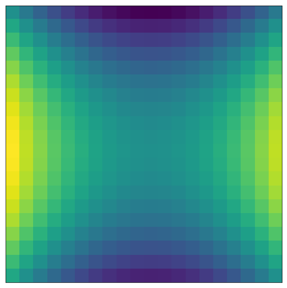
Let’s create a field following the function $f(x,y) = x^2 - y^2$.

    import matplotlib.pyplot as plt
    import numpy as np
    from numpy import ma
    %matplotlib inline
    X, Y = np.meshgrid(np.arange(-10, 10, 1), np.arange(-10, 10,1))
    field = X**2-Y**2
    plt.imshow(field);

The gradient is $\nabla f(x,y) = 2x \hat{x} - 2y \hat{y}$. We can create the parameters U and V for that hold the $\hat{x}$ and $\hat{y}$ components of the gradient, respectively, and plot them with quiver.

    U = 2*X
    V = -2*Y
    plt.imshow(field, extent=(-10.5,9.5,-10.5,9.5))
    Q = plt.quiver(X, Y, U, V, units='width')
    qk = plt.quiverkey(Q, 0.9, 0.9, 2, r'$2 \frac{m}{s}$', labelpos='E',
        coordinates='figure')

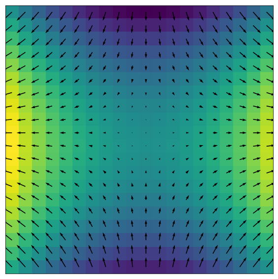
You can see the arrows are pointing from lower to higher values (darker to lighter), in the direction of the maximum positive slope.