Keras Convolutional Neural Network for CIFAR-100

1. Objective
2. Neural Networks
3. Data Augmentation
4. Activation Function
5. The Model
6. Flask and D3 App
7. Wide Neural Network?
8. Model Performance

Objective

There are standard datasets used to test new machine learning programs and compare their performance to previous models. MNIST is a set 28x28 pixel images of handwritten numbers, with 60,000 training and 10,000 test images. The CIFAR-10 and CIFAR-100 datasets consist of 32x32 pixel images in 10 and 100 classes, respectively. Both datasets have 50,000 training images and 10,000 testing images. The github repo for Keras has example Convolutional Neural Networks (CNN) for MNIST and CIFAR-10.

My goal is to create a CNN using Keras for CIFAR-100 that is suitable for an Amazon Web Services (AWS) g2.2xlarge EC2 instance. The main limitation is memory, which means the neural network can’t be as deep as other CNNs that would perform better. But creating a CNN that fits on smaller GPUs is beneficial for people who would want to use CIFAR-100 to learn how to create better neural networks, as is commonly done with MNIST and CIFAR-10.

The model and app described below are available on a GitHub repository.

Neural Networks

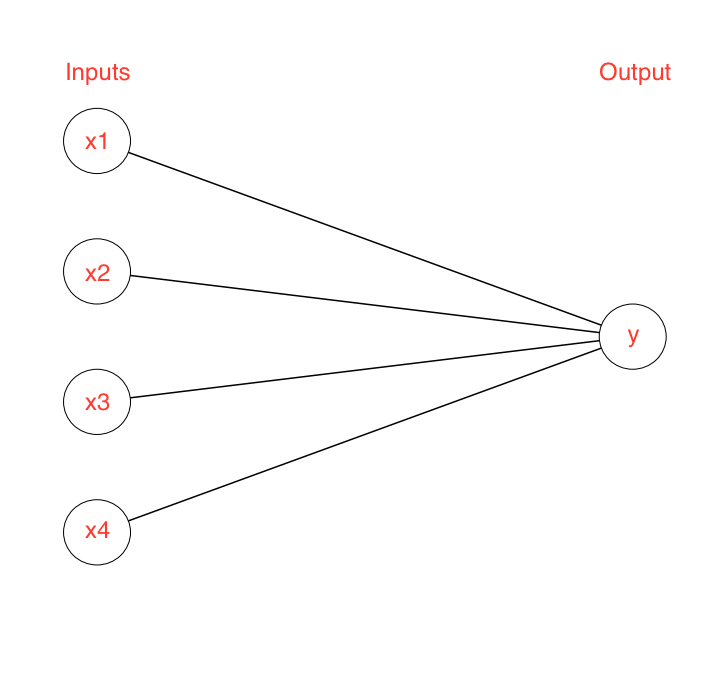
To understand neural networks, it’s easier if you think about how we recognize things. As an analogy, if you see a duck, you recognize it because it has a bill, feathers, wings, and webbed feet. So when you’re deciding if something is a duck, you have a mental checkbox that you check off. Sometimes a duck may be in water, and you can’t see the webbed feet, but you’ll still classify it as a duck because you see the bill, feathers, and wings. This is just like a regular classifier which takes in inputs ($x_1$, $x_2$, etc. would be the bill, feathers, etc.) and finds weights that predicts the classification of something most accurately ($y$ would be whether the object is a duck or not). These weights are used in the activation function, discussed below, that return a probability of the input’s classification (duck or not duck).

This relationship between the inputs and output classification can be visualized by a diagram:

But that’s not really the whole story, we need to know what a bill, feathers, wings, and webbed feet look like in the first place to know if they are there. So really, we look for edges, lines, colors, textures, and shapes that are similar to bills, feathers, wings, and webbed feet that we’ve seen before. So there’s an intermediate step between sight and classification:

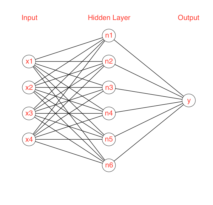
This is a basic neural network. Weights are still being applied to each of the inputs (lines, edges, etc.), and this creates new “responses” that aren’t trying to immediately predict the final class (similar to recognizing bill, feathers, etc.). These intermediate “responses” are in a hidden layer.

But that’s still not the whole story of how we recognize things. A single line or color doesn’t identify a feather, but rather a combination. So there need to be multiple hidden layers where we first identify lines, edges, etc., then a combination of those to recognize a bill, feather, etc., then a combination of those to know if we see a duck or not.

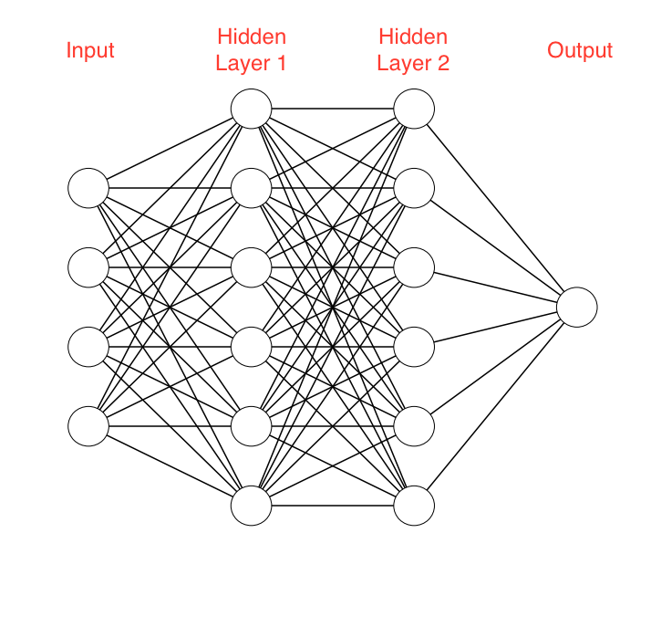
Even further, we need to recognize where the parts of the duck are relative to each other, relative sizes, etc., otherwise the duck doesn’t look like what we’re used to. More hidden layers are needed to find these relationships, and as those layers are added, the neural network is getting deeper. Deeper neural networks are able to make more complex structures in the input data.

Now, if we create a classifier to recognize a duck, it’s not necessarily going to look for the same things we do, such as feathers and an orange bill (the image may be too low resolution, or black-and-white). The features and combinations of features it looks for are whatever results in the lowest loss for the inputs its given. Also, as it searches for combinations of lines, edges, etc., what it’s looking for becomes unintelligible to us, which is why they’re called “hidden” layers.

That first layer applies filters directly to the image to search for edges, lines, colors, etc. Here’s an example illustration by Rob Fergus at NYU:

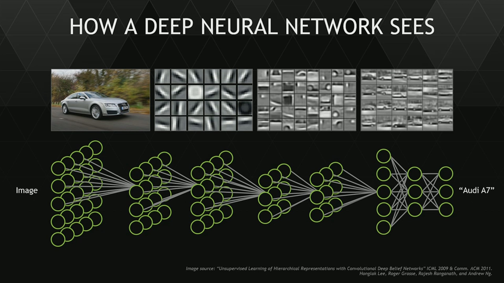
The output from this first layer is then sent to the next hidden layer, which applies new weights and filters. Here’s an illustration of how to think of a neural network recognizing a car (from Lee et al. 2011):

After the input has gone through the layers, it returns an output classification which could be incorrect. But the goal is the make the output correctly predict the classification of an object, which it won’t at first. After it has made an incorrect prediction, a backpropagation through the network updates the weights to increase the probability of returning the correct output. This process of predicting and updating the weights is repeated for new inputs, and the network learns the optimal weights that produces the most accurate model.

Data Augmentation

Object recognition is a common goal when learning machine learning and neural networks. The MNIST dataset has all of the numbers centered and cropped the same, making consistent images that can be predicted by basic models. However, object recognition becomes more difficult for images of objects that are inconsistent with each other, including shade, angle, crop size, position of object, etc.

There is a major downside to training on images that have been pre-cropped and have the objects in a consistent position: the neural network expects that the number should always be that size and in that position. It’s fast and easy to get a neural network to correctly classify a number in an image using the MNIST dataset, but that model won’t necessarily translate to detect numbers well in an arbitrary image. A (poor) fix to this problem would be to scan images, cropping the image into boxes and seeing if a number is inside that box, but that’s inefficient.

Instead, we can change the MNIST data so the numbers are no longered all centered, or the same size, or even tilted the same way. This teaches the neural network that the numbers don’t have to be that size or specific position in the image, and makes it more robust in detecting numbers in non-conforming images. (It will also expand the size of our training dataset, which is why this is called data augmentation.) While this will make the neural network take longer to train, it will make it faster and better at detecting numbers in other images.

Activation Function

A neuron’s “activation” is determined by an activation function. An example activation function is a sigmoid function which follows the relationship

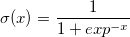
where $x$ is the dot product of the input and the weights. When $x$ is small, $\sigma$ will be closer to zero (neuron is not activated), but a large $x$ will make $\sigma$ closer to one (neuron gets activated). So a single neuron acts similar to a linear classifier.

The images are on an 8-bit grayscale with 256 intensities (in the range 0-255). Using numbers this large can result in activation saturation. Since $x$ is the dot product of the input and the weights, if the inputs are larger, the weights should be smaller. In the case of the sigmoid activation function, using initial weights that aren’t small results in the sigmoid will be forced to be one for all inputs. For this reason, the images are normalized so they are in the range 0-1 instead of 0-255 by dividing by 255.

However, even with normalization, $x$ could still be large due to other factors, such as the initial weights that are far from optimal. When this happens, the gradient is small, so even large changes in $x$ in the earlier layers may show essentially no change in the neural network’s output. This could make an important parameter or filter unlearnable. To fix this vanishing gradient problem, another common activation function is the Rectified Linear Unit (ReLU) which follows

In this case, if $x$ is less than 0, then the activation function is just zero. Otherwise, it increases linearly with $x$ and doesn’t have a maximum of one. These characteristics help the model weights converge faster, although there’s an added risk that if the learning rate is too high, a weight change could make $x$ less than zero. When this happens, there is a loss of information (can’t do gradient descent if $x$ is always zero!) that can keep $x$ permanently zero, and neurons in the network may be “dead”.

Another activiation function that has been shown to speed up the learning process and create a neural network with high accuracy over ReLUs, specifically on the CIFAR 100 dataset, is the Exponential Linear Unit (ELU; Clevert et al. 2015). The ELU follows the relationship

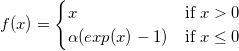
The ReLU activation function doesn’t have negative values, which results in positive mean activation, creating a bias shift in the next layers. ELUs allow negative values, bringing the mean activation closer to zero which corrects for the bias shifting and speeds up the learning. I thus used the ELU for my CNN models.

The Model

A binary class matrix is boolean, either False or True, determined by the activation function. If we used the integer value in the image, the classifier may try to do a linear fit to those numbers 0-9. Instead, for labels we can create a vector of length 10 with a one in the position of the number in the image, and zeros elsewhere.

# convert class vectors to binary class matrices
y_train = keras.utils.to_categorical(y_train, num_classes)
y_test = keras.utils.to_categorical(y_test, num_classes)

Now for the structure of the neural network! The CNN is first set to be sequential (and every layer after is inferred to be sequantial).

model = Sequential()

The first stack has two convolutional layers with 128 units. Pooling is done by looking at a grid (here a 2x2 grid) and only using the maximum. This removes the number of parameters used and leaves only the most significant ones to prevent overfitting, with the added benefit of reducing the amount of memory needed for the network. A dropout is then used to further prevent overfitting by setting any fractional input rates at or below the dropout value to zero. This will remove neurons in the network, leaving behind only neural connections with heavier weights.

    model.add(Conv2D(128, (3, 3), padding='same',
        input_shape=x_train.shape[1:]))
    model.add(Activation('elu'))
    model.add(Conv2D(128, (3, 3)))
    model.add(Activation('elu'))
    model.add(MaxPooling2D(pool_size=(2, 2)))
    model.add(Dropout(0.1))

Continuing to two following stacks with 2x2 pooling and dropouts after each:

    model.add(Conv2D(256, (3, 3), padding='same'))
    model.add(Activation('elu'))
    model.add(Conv2D(256, (3, 3)))
    model.add(Activation('elu'))
    model.add(MaxPooling2D(pool_size=(2, 2)))
    model.add(Dropout(0.25))

    model.add(Conv2D(512, (3, 3), padding='same'))
    model.add(Activation('elu'))
    model.add(Conv2D(512, (3, 3)))
    model.add(Activation('elu'))
    model.add(MaxPooling2D(pool_size=(2, 2)))
    model.add(Dropout(0.5))

The neural network ultimately needs to output the probability of the different classes in an array. After the convolution stacks, the probabilities need to be flattened to a 1D feature vector. The dense layers are fully-connected layers that apply transformations and change the dimensions. The final dense layer needs to be the same length as the number of classes, and gives the probability of each class.

    model.add(Flatten())
    model.add(Dense(1024))
    model.add(Activation('elu'))
    model.add(Dropout(0.5))
    model.add(Dense(100))
    model.add(Activation('softmax'))

Flask and D3 App

I made a basic app that takes in an online image and use the CNN model to predict what the image was. It used Flask, which is used to make python-based webpages, and D3, a JavaScript library used to create visuals. After inputting the URL of the image, it returns a graph showing the probabilities of the top five predictions. (Higher-resolution on YouTube).

The image used:

The prediction:

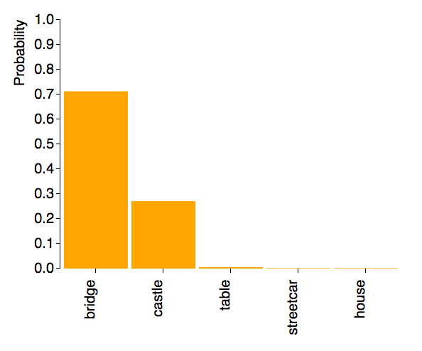
Although the model was trained to recognize images of single objects, it was able to recognize both the bridge and the castle.

Wide Neural Network?

The Keras example CNN for CIFAR 10 has four convolutional layers. The first two have 32 filters, second two have 64 filters. In creating a CNN for CIFAR 100, I initially attempted to increase accuracy by making it deeper with more hidden layers. However, after grid searching different parameters such as learning rates adn decays, batch sizes, activation functions, etc., I was only able to get a maximum accuracy of 0.55 when adding two more layers.

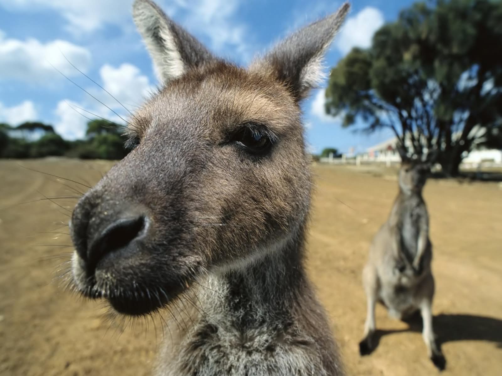
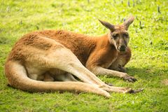
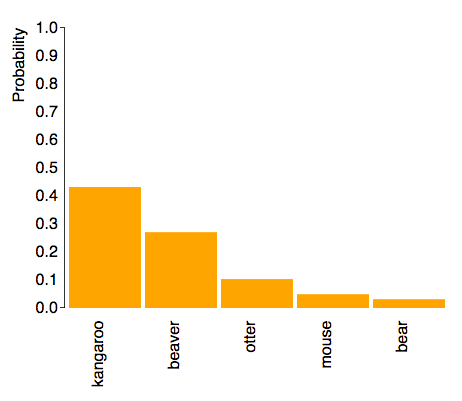
In searching through predictions for images, I tested various images of kangaroos and it was accurate on most of them, until I tested on a kangaroo that is grayer than the others:

Resized image for prediction:

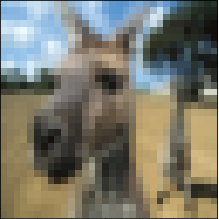
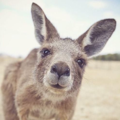
This image had the following predictions:

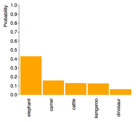
This kangaroo was predicted to be an elephant. It is similar in shape to other kangaroos that the model had recognized accurately, but only grayer in color. This indicated a potential issue that the model was putting emphasis on color rather than shape, possibly due to the number of filters being used in the first layers.

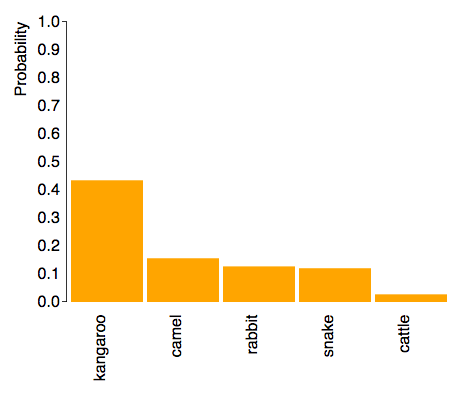
Different objects have similar structure elements (i.e. vertical/horizontal/slanted edges, colors, etc.), but 32 filters is not sufficient for the 100 different classes of objects. I increased the first two layers from 32 to 128 filters, and the next two layers from 64 to 256, and the prediction for the image above changed to:

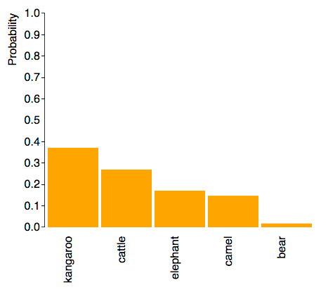
Now the highest prediction is a kangaroo. This shows that the while a deeper network enables it to recognize more complicated structures, it’s necessary not to limit the number of structures that can be used.

Model Performance

The final model had a validation accuracy of 0.64, which depends on the probability of the predictions, when predicting on the test images. When considering simply how many “guesses” it would take for the model to get the object correct, it got 65% of objects correct in one guess, 77% in two guesses, and 83% in three guesses.

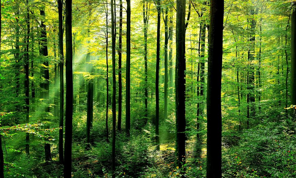
Naturally, it gets some things completely wrong. For example, in this image it wasn’t able to identify the forest or the chimpanzee, both objects it should recognize.

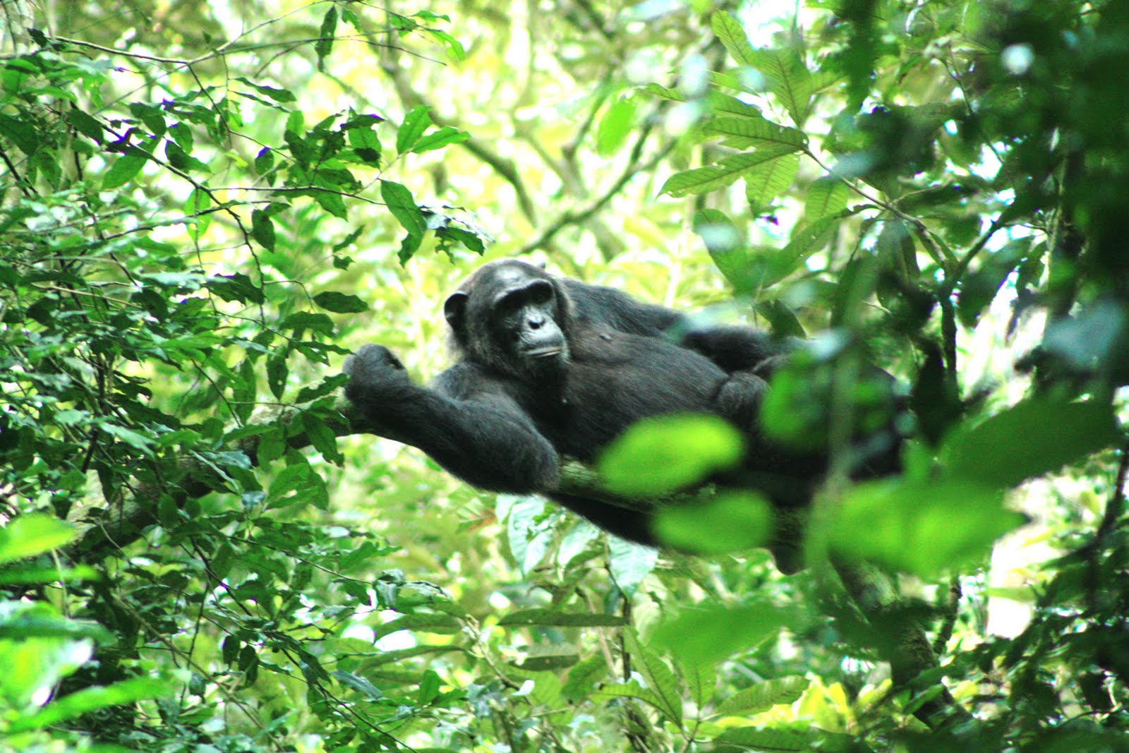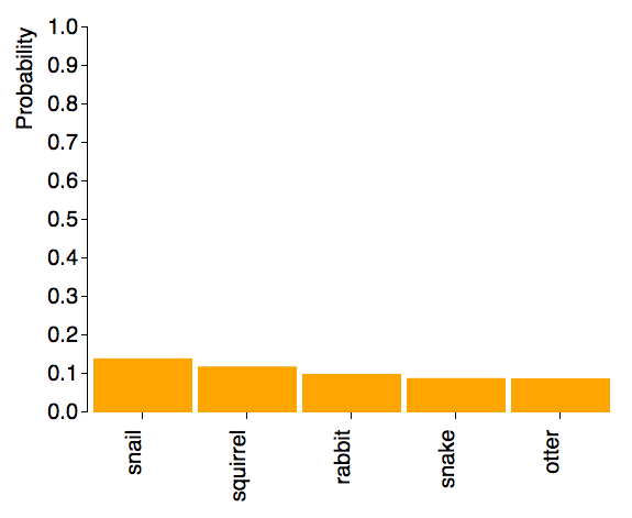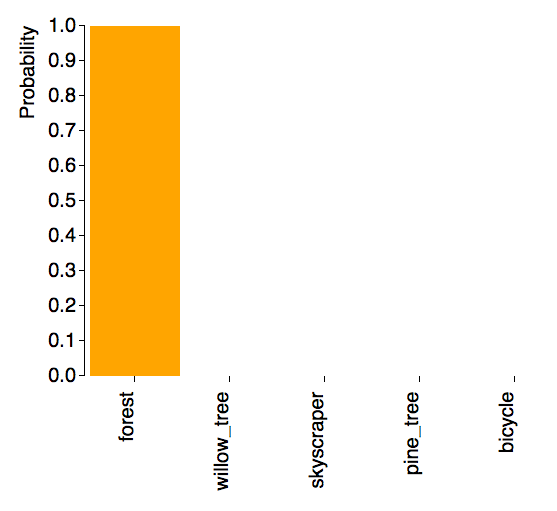
What the CNN is able to predict does depend on what images were input. For example, if “forest” images showed the base of trees (unlike above), then it wouldn’t be able to recognize this as a forest. If it’s only been trained on chimpanzees where they are the main focus of the image, it will have a harder time detecting the chimpanzee when it’s a smaller part of the image. As can be seen here, the predictor easily identified a close-up of a chimpanzee and a forest with tree bases:

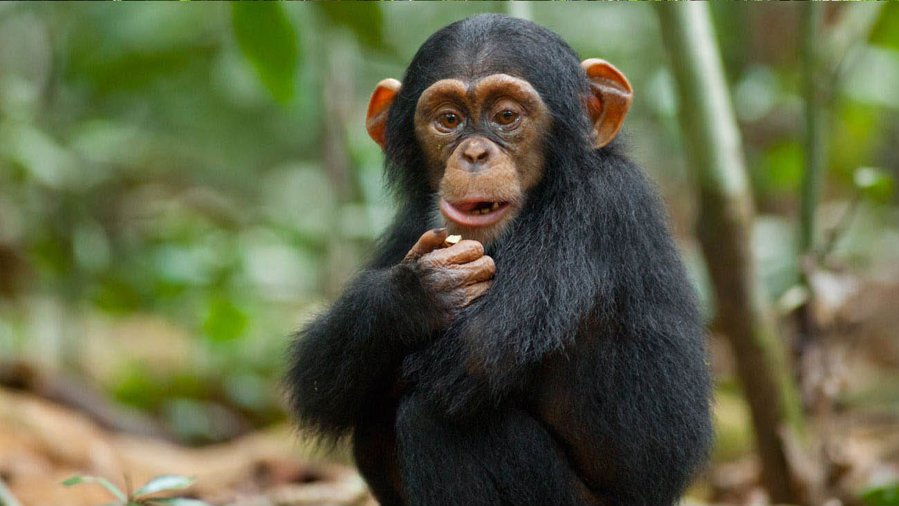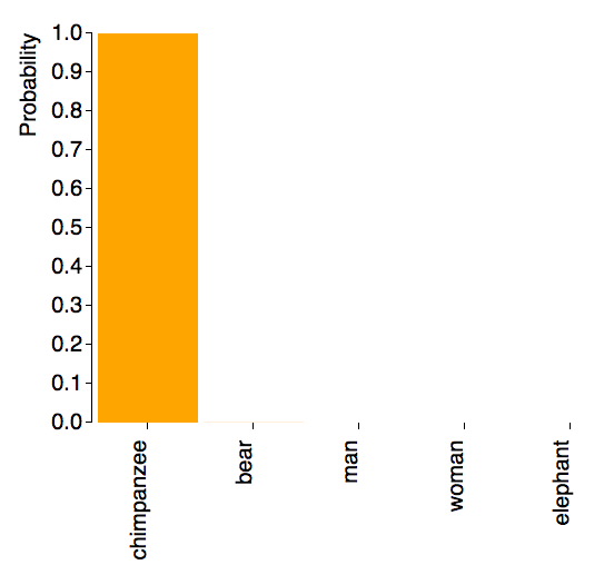As expected, the model is able to classify objects correctly even when their features were displayed differently. For example, the following are three kangaroos in completely different positions it correctly classified:

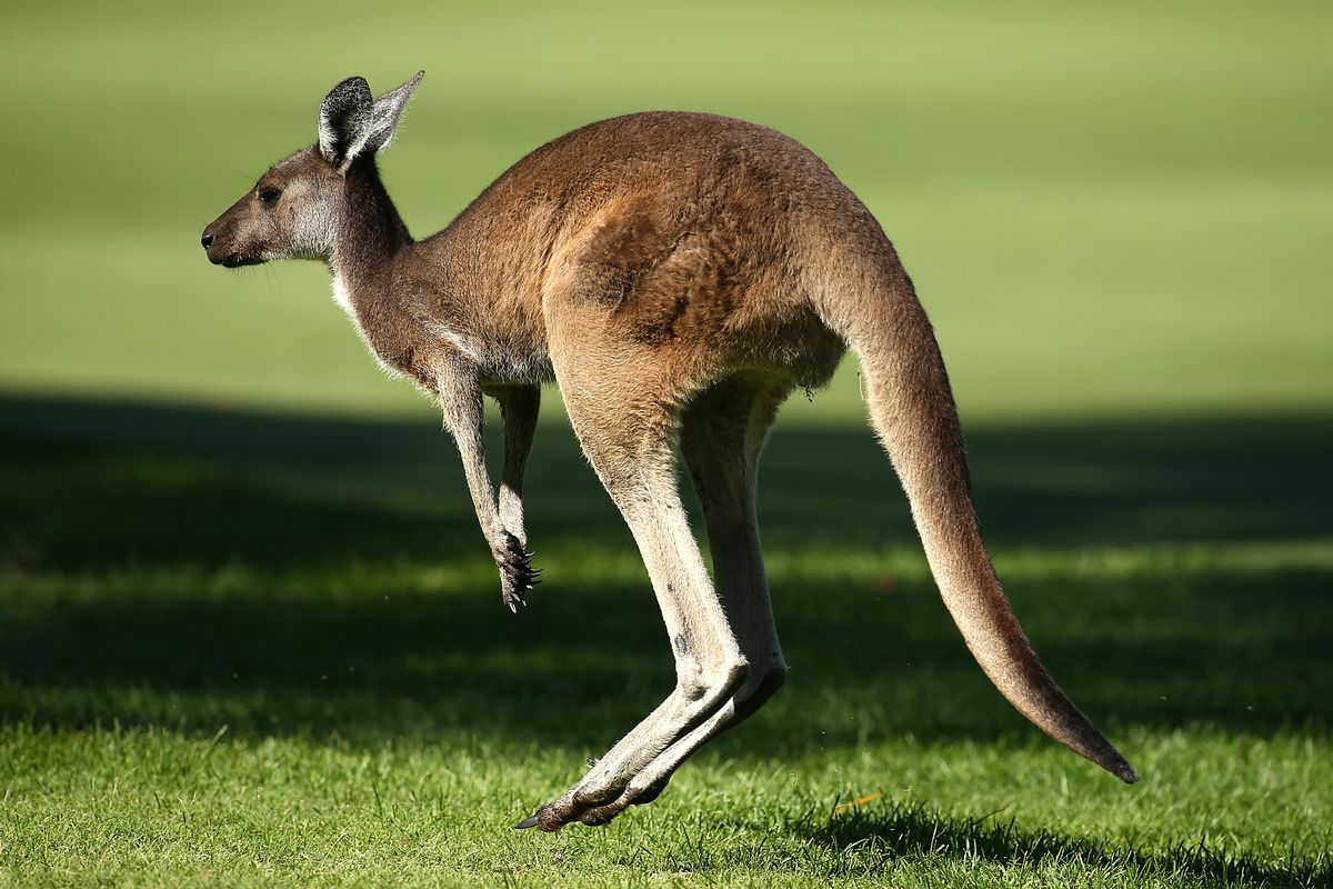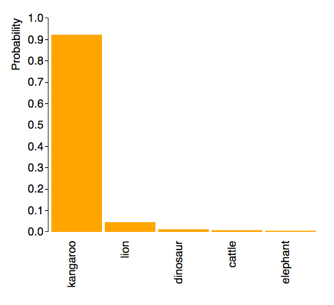It is also able to distinguish between things that have similar features, for example the difference between my younger daughter when she a “baby” and my older daughter as a “girl”.

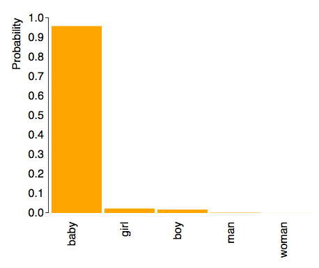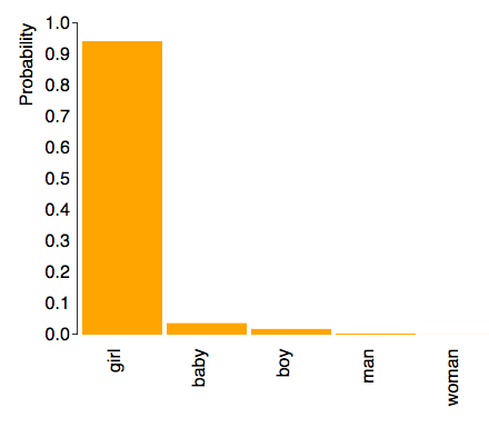As shown above in the video, it can identify multiple objects in the image. Another example is this house in the mountains:
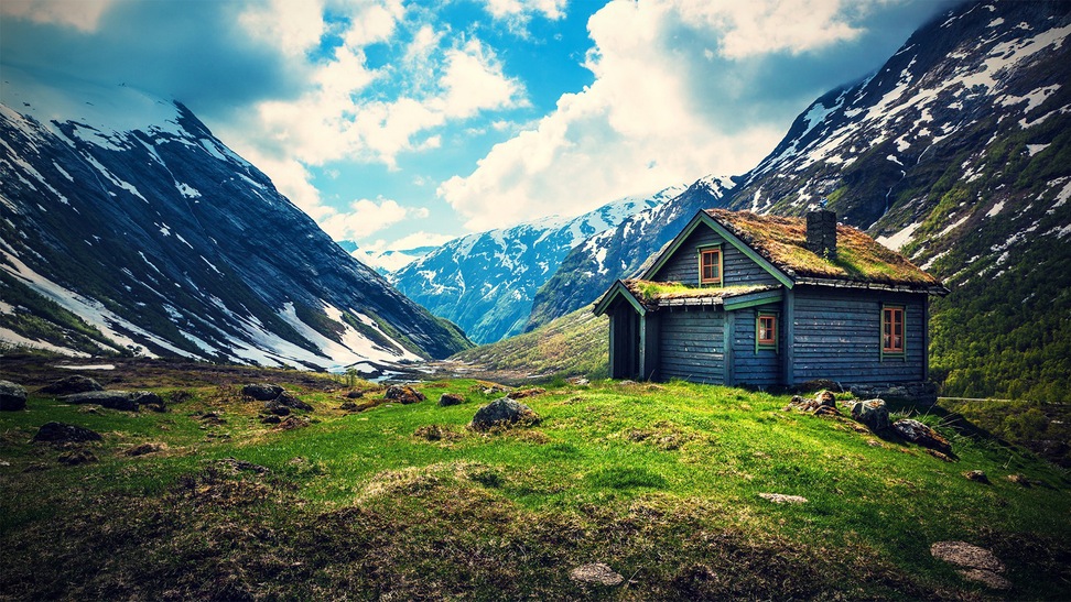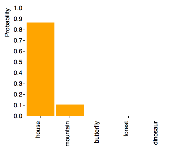